Simulation add-operation with pytorch

We all know that the theory Universal approximate theorem, said that a linear layer can simulate all function in theory. But in fact, we can not guaranteed that the training algorithm will be able to learn that function. The first reason is optimization algorithm can not find it. It also may caused by finding wrong function for overfitting.

But in this article, we will challenge this theory, at least with our simply function such as adding. On the way to the training of model, we also overcome so many difficulties. Now let’s begin our novel travel.

1.Task

In this section, we will challenge it by simulate add function. In detail, we will use linear layers to approximate function:

The n is the number of numbers to add together. In other words, the input’s dimension is batch_size * n. We split our codes into two source files: main.py, model.py. click them to view the source codes.

2.Dataset

What we use is a famous dataset named toy dataset. All datas are generated randomly between [0, 1) in this dataset. We suppose X is the input of neural network, and L is the augment paramenter, so our input datas is:

The L is a hyperparameter, and it makes our input numbers range from -L to L inclusive.

3.Model

We suppose our input is a variable:

in which the batch_size is the batch size of our input to decreasing the fluctuate in training stage. the n is the number we explain in sction 1.Task, the amount of numbers to add together. Than we send them into the linear network, and get a [batch_size * 1] variable finally. In every epoch, we split all datas into several batches that are sended into network to training one by one.

For our goal is simulating a function in base linear layer, so our model is built by custom layers. In this way, we can add L1 normalization, L2 normalization and bias in our will. I believe we can know what happen indeed in this way.

The following is the our linear layer:

class linear(Function):

    @staticmethod
    def forward(self, input, weight, bias):
        '''
        input.shape = (n, m)
        weight.shape = (m, k)
        bias.shape = (1, )
        output.shape = (n, k)
        '''
        self.save_for_backward(input, weight)
        output = input.mm(weight) + bias
        return output

    @staticmethod
    def backward(self, grad_output):
        '''
        grad_output.shape = (n, k)
        grad_input.shape = (n, m)
        grad_weight.shape = (m, k)
        grad_bias = (1, )
        '''
        input, weight = self.saved_variables
        return grad_output.mm(weight.t()), input.t().mm(grad_output), torch.sum(grad_output)

The input Variable X is processed by the first linear layer, and we choose tanh as our activation function. If we do not choose one activation, the model will become

It obvious that the two layer model will equal to the model which just has one linear layer. In other words, we add one activation function to the model to increasing the capacity the model. The practice of our training show that it seems not bad at least!

So our full model:

class model(nn.Module):

    def __init__(self, config):
        super(model, self).__init__()
        
        self.config = config

        self.weight1 = nn.Parameter(torch.randn(self.config['n'], self.config['hidden']))
        self.bias1 = nn.Parameter(torch.randn(1))
        self.weight2 = nn.Parameter(torch.randn(self.config['hidden'], 1))
        self.bias2 = nn.Parameter(torch.randn(1))

        self.linear1 = linear.apply
        self.linear2 = linear.apply

    def forward(self, x):

        x = F.tanh(self.linear1(x, self.weight1, self.bias1))
        x = self.linear2(x, self.weight2, self.bias2)

        return x

Note that we add a bias to every linear layer. I think god may know whether it is necessary.

3.Explore

We firstly choose MSE as our loss function, and set learning_rate to 0.001. The traing detail:

    for epoch in range(1, self.config['epoch'] + 1):

        total_loss = 0
        self.loadBatches()
        for batch in self.batches:
            x = [b[0] for b in batch]
            label = [b[1] for b in batch]
            
            x = Variable(torch.Tensor(x))
            label = Variable(torch.Tensor(label)).t()

            self.optimizer.zero_grad()
            y = self.model(x)
            loss = torch.sum((y - label.squeeze()) ** 2)
            total_loss += loss.data.numpy()[0]
            loss.backward()
            self.optimizer.step()

As we can see in above code, we send all datas to train one time in every epoch. We use MSE loss function, and although not clearly, we use Adam to optimizer the loss function in training phase. We train about 200 epoch in this way with 0.001 learing_rate, the result show:

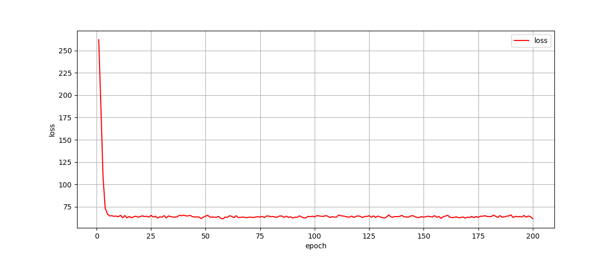
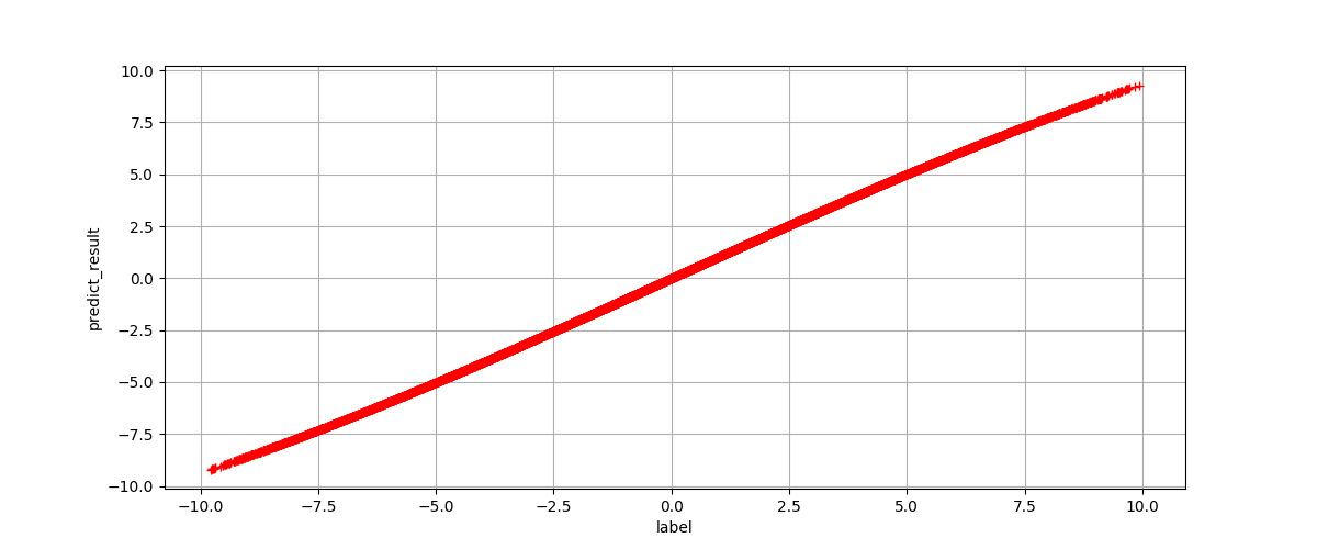
It obvious that our network not perform well as we expected! If there is someone one doubt that the network has in convergence, we will reveal the output of the network. For more clearly showing, we draw all output values and labels, and compare the distance between them:

Take care of the value of x axes and y axes. By comparing them, we can conclude that our network dose not learn right add operation at all.

So why?

Let’s observe the code in our training phase:

    for epoch in range(1, self.config['epoch'] + 1):

        for batch in self.batches:
            ...
            
            y = self.model(x)
            loss = torch.sum((y - label.squeeze()) ** 2)
            
            ...

In fact, it’s really strange that our code can run with no error! In our model, with (batch_size, n) of input, and (batch_size, 1) output. In other words, the shape of y in above code is (batch_size, 1). But the shape of label in above code is (batch_size, ). Now we change our code to:

for epoch in range(1, self.config['epoch'] + 1):

    total_loss = 0
    self.loadBatches()
    for batch in self.batches:
        x = [b[0] for b in batch]
        label = [b[1] for b in batch]

        x = Variable(torch.Tensor(x))
        label = Variable(torch.Tensor(label)).t()

        self.optimizer.zero_grad()
        y = self.model(x)
        loss = torch.sum((y.t() - label) ** 2)

        total_loss += loss.data.numpy()[0]
        loss.backward()
        self.optimizer.step()

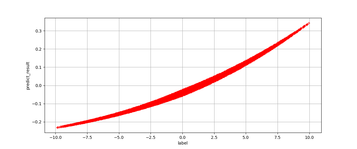
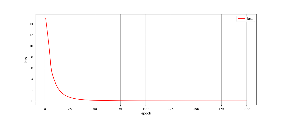
We get the expected result in this way:

Conclude

We use two custom linear layer to simulate add operation in this article. Firstly our network did not learn the right function, for our wrong loss function lead to wrong gradient to backward. We rectify it and get the right result.

But I am so sorry that we have no time to try more parameters and more models. However I still believe it will work if we set the good enough parameters.